MS Data

Spectrum

The most important container for raw data and peaks is MSSpectrum which we have already worked with in the Getting Started tutorial. MSSpectrum is a container for 1-dimensional peak data (a container of Peak1D). You can access these objects directly, however it is faster to use the get_peaks() and set_peaks functions which use Python numpy arrays for raw data access. Meta-data is accessible through inheritance of the SpectrumSettings objects which handles meta data of a spectrum.

In the following example program, a MSSpectrum is filled with peaks, sorted according to mass-to-charge ratio and a selection of peak positions is displayed.

First we create a spectrum and insert peaks with descending mass-to-charge ratios:

from pyopenms import *
spectrum = MSSpectrum()
mz = range(1500, 500, -100)
i = [0 for mass in mz]
spectrum.set_peaks([mz, i])

# Sort the peaks according to ascending mass-to-charge ratio
spectrum.sortByPosition()

# Iterate over spectrum of those peaks
for p in spectrum:
  print(p.getMZ(), p.getIntensity())

# More efficient peak access with get_peaks()
for mz, i in zip(*spectrum.get_peaks()):
  print(mz, i)

# Access a peak by index
print(spectrum[2].getMZ(), spectrum[2].getIntensity())

Note how lines 11-12 (as well as line 19) use the direct access to the Peak1D objects (explicit iteration through the MSSpectrum object, which is convenient but slow since a new Peak1D object needs to be created each time) while lines 15-16 use the faster access through numpy arrays. Direct iteration is only shown for demonstration purposes and should not be used in production code.

To discover the full set of functionality of MSSpectrum, we use the help() function. In particular, we find several important sets of meta information attached to the spectrum including retention time, the ms level (MS1, MS2, …), precursor ion, ion mobility drift time and extra data arrays.

help(MSSpectrum)

We now set several of these properties in a current MSSpectrum:

# create spectrum and set properties
spectrum = MSSpectrum()
spectrum.setDriftTime(25) # 25 ms
spectrum.setRT(205.2) # 205.2 s
spectrum.setMSLevel(3) # MS3

# Add peak(s) to spectrum
spectrum.set_peaks( ([401.5], [900]) )

# create precursor information
p = Precursor()
p.setMZ(600) # isolation at 600 +/- 1.5 Th
p.setIsolationWindowLowerOffset(1.5)
p.setIsolationWindowUpperOffset(1.5)
p.setActivationEnergy(40) # 40 eV
p.setCharge(4) # 4+ ion

# and store precursor in spectrum
spectrum.setPrecursors( [p] )

# set additional instrument settings (e.g. scan polarity)
IS = InstrumentSettings()
IS.setPolarity(IonSource.Polarity.POSITIVE)
spectrum.setInstrumentSettings(IS)

# get and check scan polarity
polarity = spectrum.getInstrumentSettings().getPolarity()
if (polarity == IonSource.Polarity.POSITIVE):
  print("scan polarity: positive")
elif (polarity == IonSource.Polarity.NEGATIVE):
  print("scan polarity: negative")

# Optional: additional data arrays / peak annotations
fda = FloatDataArray()
fda.setName("Signal to Noise Array")
fda.push_back(15)
sda = StringDataArray()
sda.setName("Peak annotation")
sda.push_back("y15++")
spectrum.setFloatDataArrays( [fda] )
spectrum.setStringDataArrays( [sda] )

# Add spectrum to MSExperiment
exp = MSExperiment()
exp.addSpectrum(spectrum)

# Add second spectrum to the MSExperiment
spectrum2 = MSSpectrum()
spectrum2.set_peaks( ([1, 2], [1, 2]) )
exp.addSpectrum(spectrum2)

# store spectra in mzML file
MzMLFile().store("testfile.mzML", exp)

We have created a single spectrum and set basic spectrum properties (drift time, retention time, MS level, precursor charge, isolation window and activation energy). Additional instrument settings allow to set e.g. the polarity of the Ion source). We next add actual peaks into the spectrum (a single peak at 401.5 m/z and 900 intensity). Additional metadata can be stored in data arrays for each peak (e.g. use cases care peak annotations or “Signal to Noise” values for each peak. Finally, we add the spectrum to an MSExperiment container to save it using the MzMLFile class in a file called “testfile.mzML”.

You can now open the resulting spectrum in a spectrum viewer. We use the OpenMS viewer TOPPView (which you will get when you install OpenMS from the official website) and look at our spectrum:

TOPPView displays our spectrum with its single peak at 401.5 m/z and it also correctly displays its retention time at 205.2 seconds and precursor isolation target of 600.0 m/z. Notice how TOPPView displays the information about the S/N for the peak (S/N = 15) and its annotation as y15++ in the status bar below when the user clicks on the peak at 401.5 m/z as shown in the screenshot.

We can also visualize our spectrum with matplotlib using the following function:

 import matplotlib.pyplot as plt

 def plot_spectrum(spectrum):
     # plot every peak in spectrum and annotate with it's m/z
     for mz, i in zip(*spectrum.get_peaks()):
         plt.plot([mz, mz], [0, i], color = 'black')
         plt.text(mz, i, str(mz))

     # for the title add RT and Precursor m/z if available
     title = ''
     if spectrum.getRT() >= 0:
         title += 'RT: ' + str(spectrum.getRT())
     if len(spectrum.getPrecursors()) >= 1:
         title += '   Precursor m/z: ' + str(spectrum.getPrecursors()[0].getMZ())

     plt.title(title)
     plt.ylabel('intensity')
     plt.xlabel('m/z')
     plt.ylim(bottom=0)

     plt.show()

# plotting out spectrum that was defined earlier
plot_spectrum(spectrum)

Chromatogram

An additional container for raw data is the MSChromatogram container, which is highly analogous to the MSSpectrum container, but contains an array of ChromatogramPeak and is derived from ChromatogramSettings:

import numpy as np

def gaussian(x, mu, sig):
    return np.exp(-np.power(x - mu, 2.) / (2 * np.power(sig, 2.)))

# Create new chromatogram
chromatogram = MSChromatogram()

# Set raw data (RT and intensity)
rt = range(1500, 500, -100)
i = [gaussian(rtime, 1000, 150) for rtime in rt]
chromatogram.set_peaks([rt, i])

# Sort the peaks according to ascending retention time
chromatogram.sortByPosition()

# Iterate over chromatogram of those peaks
for p in chromatogram:
    print(p.getRT(), p.getIntensity())

# More efficient peak access with get_peaks()
for rt, i in zip(*chromatogram.get_peaks()):
    print(rt, i)

# Access a peak by index
print(chromatogram[2].getRT(), chromatogram[2].getIntensity())

# Add meta information to the chromatogram
chromatogram.setNativeID("Trace XIC@405.2")

# Store a precursor ion for the chromatogram
p = Precursor()
p.setIsolationWindowLowerOffset(1.5)
p.setIsolationWindowUpperOffset(1.5)
p.setMZ(405.2) # isolation at 405.2 +/- 1.5 Th
p.setActivationEnergy(40) # 40 eV
p.setCharge(2) # 2+ ion
p.setMetaValue("description", chromatogram.getNativeID())
p.setMetaValue("peptide_sequence", chromatogram.getNativeID())
chromatogram.setPrecursor(p)

# Also store a product ion for the chromatogram (e.g. for SRM)
p = Product()
p.setMZ(603.4) # transition from 405.2 -> 603.4
chromatogram.setProduct(p)

# Store as mzML
exp = MSExperiment()
exp.addChromatogram(chromatogram)
MzMLFile().store("testfile3.mzML", exp)

# Visualize the resulting data using matplotlib
import matplotlib.pyplot as plt

for chrom in exp.getChromatograms():
    retention_times, intensities = chrom.get_peaks()
    plt.plot(retention_times, intensities, label = chrom.getNativeID())

plt.xlabel('time (s)')
plt.ylabel('intensity (cps)')
plt.legend()
plt.show()

This shows how the MSExperiment class can hold spectra as well as chromatograms.

Again we can visualize the resulting data using TOPPView using its chromatographic viewer capability, which shows the peak over retention time:

Note how the annotation using precursor and production mass of our XIC chromatogram is displayed in the viewer.

We can also visualize the resulting data using matplotlib. Here we can plot every chromatogram in our MSExperiment and label it with it’s native ID.

LC-MS/MS Experiment

In OpenMS, LC-MS/MS injections are represented as so-called peak maps (using the MSExperiment class), which we have already encountered above. The MSExperiment class can hold a list of MSSpectrum object (as well as a list of MSChromatogram objects, see below). The MSExperiment object holds such peak maps as well as meta-data about the injection. Access to individual spectra is performed through MSExperiment.getSpectrum and MSExperiment.getChromatogram.

In the following code, we create an MSExperiment and populate it with several spectra:

# The following examples creates an MSExperiment which holds six
# MSSpectrum instances.
exp = MSExperiment()
for i in range(6):
    spectrum = MSSpectrum()
    spectrum.setRT(i)
    spectrum.setMSLevel(1)
    for mz in range(500, 900, 100):
      peak = Peak1D()
      peak.setMZ(mz + i)
      peak.setIntensity(100 - 25*abs(i-2.5) )
      spectrum.push_back(peak)
    exp.addSpectrum(spectrum)

# Iterate over spectra
for spectrum in exp:
    for peak in spectrum:
        print (spectrum.getRT(), peak.getMZ(), peak.getIntensity())

In the above code, we create six instances of MSSpectrum (line 4), populate it with three peaks at 500, 900 and 100 m/z and append them to the MSExperiment object (line 13). We can easily iterate over the spectra in the whole experiment by using the intuitive iteration on lines 16-18 or we can use list comprehensions to sum up intensities of all spectra that fulfill certain conditions:

# Sum intensity of all spectra between RT 2.0 and 3.0
print(sum([p.getIntensity() for s in exp if s.getRT() >= 2.0 and s.getRT() <= 3.0 for p in s]))

700.0
87.5 * 8
700.0

We could store the resulting experiment containing the six spectra as mzML using the MzMLFile object:

# Store as mzML
MzMLFile().store("testfile2.mzML", exp)

Again we can visualize the resulting data using TOPPView using its 3D viewer capability, which shows the six scans over retention time where the traces first increase and then decrease in intensity:

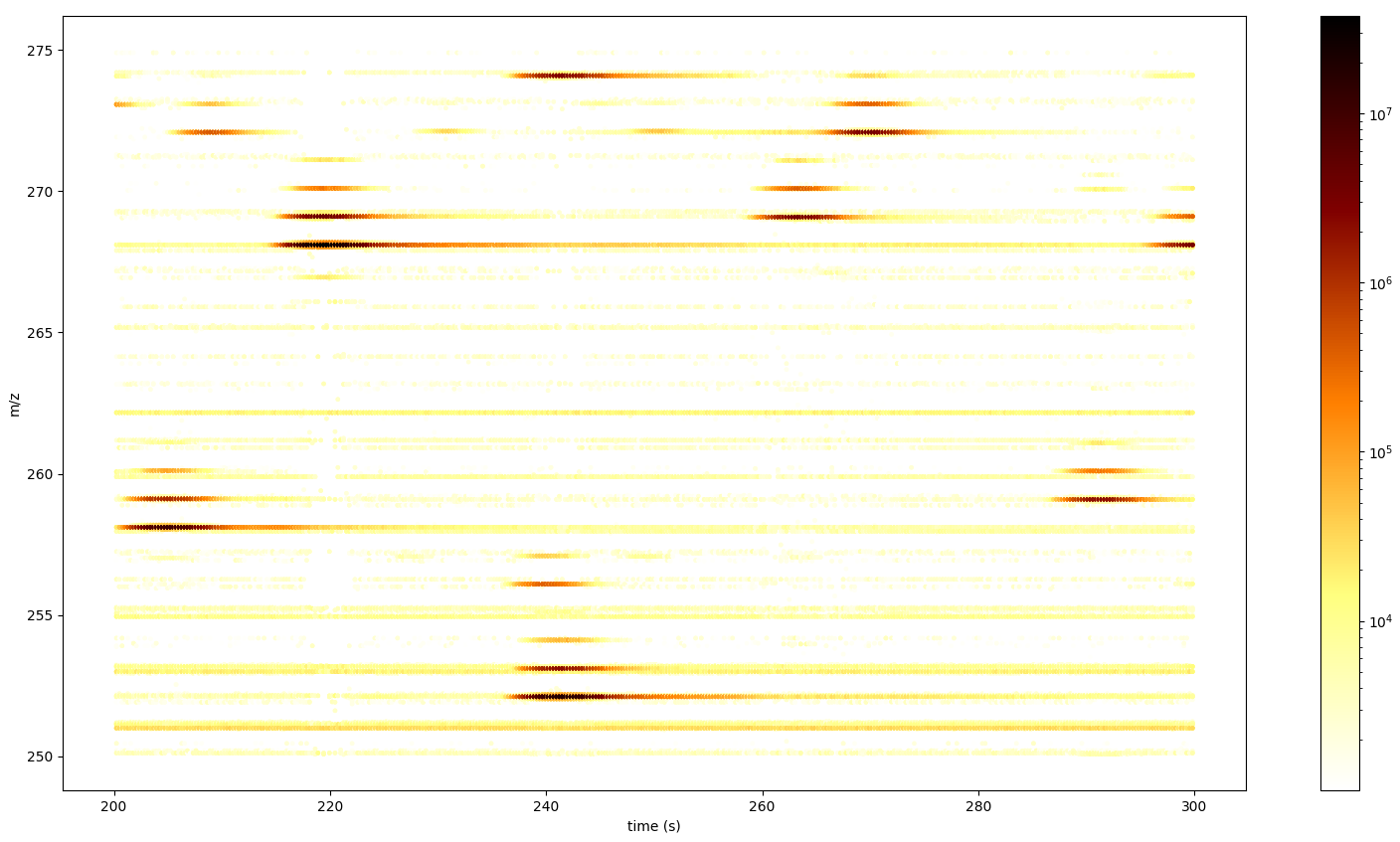
Alternatively we can visualize our data directly with Python. For smaller data sets we can use matplotlib to generate a 2D scatter plot with the peak intensities represented by a colorbar. With this plot we can zoom in and inspect our data in more detail.

The following example figures were generated using a mzML file provided by OpenMS.

 import numpy as np
 import matplotlib.pyplot as plt
 import matplotlib.colors as colors

 def plot_spectra_2D(exp, ms_level=1, marker_size = 5):
     exp.updateRanges()
     print('collecting peak data...')
     for spec in exp:
         if spec.getMSLevel() == ms_level:
             mz, intensity = spec.get_peaks()
             p = intensity.argsort() # sort by intensity to plot highest on top
             rt = np.full([mz.shape[0]], spec.getRT(), float)
             plt.scatter(rt, mz[p], c = intensity[p], cmap = 'afmhot_r', s=marker_size,
                         norm=colors.LogNorm(exp.getMinIntensity()+1, exp.getMaxIntensity()))
     plt.clim(exp.getMinIntensity()+1, exp.getMaxIntensity())
     plt.xlabel('time (s)')
     plt.ylabel('m/z')
     plt.colorbar()
     print('showing plot...')
     plt.show() # slow for larger data sets

from urllib.request import urlretrieve

gh = "https://raw.githubusercontent.com/OpenMS/pyopenms-docs/master"
urlretrieve (gh + "/src/data/FeatureFinderMetaboIdent_1_input.mzML", "test.mzML")

exp = MSExperiment()
MzMLFile().load('test.mzML', exp)

plot_spectra_2D(exp)

For larger data sets this will be too slow since every individual peak gets displayed. However, we can use BilinearInterpolation which produces an overview image of our spectra. This can be useful for a brief visual inspection of your sample in quality control.

 import numpy as np
 import matplotlib.pyplot as plt

 def plot_spectra_2D_overview(experiment):
     rows = 200.0
     cols = 200.0
     exp.updateRanges()

     bilip = BilinearInterpolation()
     tmp = bilip.getData()
     tmp.resize(int(rows), int(cols), float())
     bilip.setData(tmp)
     bilip.setMapping_0(0.0, exp.getMinRT(), rows-1, exp.getMaxRT())
     bilip.setMapping_1(0.0, exp.getMinMZ(), cols-1, exp.getMaxMZ())
     print('collecting peak data...')
     for spec in exp:
         if spec.getMSLevel() == 1:
             mzs, ints = spec.get_peaks()
             rt = spec.getRT()
             for i in range(0, len(mzs)):
                 bilip.addValue(rt, mzs[i], ints[i])

     data = np.ndarray(shape=(int(cols), int(rows)), dtype=np.float64)
     for i in range(int(rows)):
         for j in range(int(cols)):
             data[i][j] = bilip.getData().getValue(i,j)

     plt.imshow(np.rot90(data), cmap='gist_heat_r')
     plt.xlabel('retention time (s)')
     plt.ylabel('m/z')
     plt.xticks(np.linspace(0,int(rows),20, dtype=int),
             np.linspace(exp.getMinRT(),exp.getMaxRT(),20, dtype=int))
     plt.yticks(np.linspace(0,int(cols),20, dtype=int),
             np.linspace(exp.getMinMZ(),exp.getMaxMZ(),20, dtype=int)[::-1])
     print('showing plot...')
     plt.show()

plot_spectra_2D_overview(exp)

Example: Precursor Purity

When an MS/MS spectrum is generated, the precursor from the MS1 spectrum is gathered, fragmented and measured. In practice, the instrument gathers the ions in a user-defined window around the precursor m/z - the so-called precursor isolation window.

In some cases, the precursor isolation window contains contaminant peaks from other analytes. Depending on the analysis requirements, this can lead to issues in quantification for example, for isobaric experiments.

Here, we can assess the purity of the precursor to filter spectra with a score below our expectation.

from urllib.request import urlretrieve

gh = "https://raw.githubusercontent.com/OpenMS/pyopenms-docs/master"
urlretrieve (gh + "/src/data/PrecursorPurity_input.mzML", "PrecursorPurity_input.mzML")

exp = MSExperiment()
MzMLFile().load("PrecursorPurity_input.mzML", exp)

# for this example, we check which are MS2 spectra and choose one of them
for element in exp:
    print(element.getMSLevel())

# get the precursor information from the MS2 spectrum at index 3
ms2_precursor = Precursor()
ms2_precursor = exp[3].getPrecursors()[0];

# get the previous recorded MS1 spectrum
isMS1 = False;
i = 3 # start at the index of the MS2 spectrum
while isMS1 == False:
    if exp[i].getMSLevel() == 1:
        isMS1 = True
    else:
        i -= 1

ms1_spectrum = exp[i]

# calculate the precursor purity in a 10 ppm precursor isolation window
purity_score = PrecursorPurity().computePrecursorPurity(ms1_spectrum, ms2_precursor, 10, True)

print(purity_score.total_intensity) # 9098343.890625
print(purity_score.target_intensity) # 7057944.0
print(purity_score.signal_proportion) # 0.7757394186070014
print(purity_score.target_peak_count) # 1
print(purity_score.residual_peak_count) # 4

We could assess that we have four other non-isotopic peaks apart from our precursor and its isotope peaks within our precursor isolation window. The signal of the isotopic peaks correspond to roughly 78% of all intensities in the precursor isolation window.

Example: Filtering Spectra

Here we will look at some code snippets that might come in handy when dealing with spectra data.

But first, we will load some test data:

gh = "https://raw.githubusercontent.com/OpenMS/pyopenms-docs/master"
urlretrieve (gh + "/src/data/tiny.mzML", "test.mzML")

inp = MSExperiment()
MzMLFile().load("test.mzML", inp)

Filtering Spectra by MS level

We will filter the data from “test.mzML” file by only retaining only spectra that are not MS1 spectra (e.g.MS2, MS3 or MSn spectra):

filtered = MSExperiment()
for s in inp:
    if s.getMSLevel() > 1:
        filtered.addSpectrum(s)

# filtered now only contains spectra with MS level > 2

Filtering by scan number

We could also use a list of scan numbers as filter criterium to only retain a list of MS scans we are interested in:

scan_nrs = [0, 2, 5, 7]

filtered = MSExperiment()
for k, s in enumerate(inp):
  if k in scan_nrs:
    filtered.addSpectrum(s)

Filtering Spectra and Peaks

Suppose we are interested in only in a small m/z window of our fragment ion spectra. We can easily filter our data accordingly:

mz_start = 6.0
mz_end = 12.0
filtered = MSExperiment()
for s in inp:
  if s.getMSLevel() > 1:
    filtered_mz = []
    filtered_int = []
    for mz, i in zip(*s.get_peaks()):
      if mz > mz_start and mz < mz_end:
        filtered_mz.append(mz)
        filtered_int.append(i)
    s.set_peaks((filtered_mz, filtered_int))
    filtered.addSpectrum(s)

  # filtered only contains only fragment spectra with peaks in range [mz_start, mz_end]

Note that in a real-world application, we would set the mz_start and mz_end parameter to an actual area of interest, for example the area between 125 and 132 which contains quantitative ions for a TMT experiment.

Similarly we could only retain peaks above a certain intensity or keep only the top N peaks in each spectrum.

For more advanced filtering tasks pyOpenMS provides special algorithm classes. We will take a closer look at some of them in the algorithm section.